
Diffusion Models from Scratch: The Math and Code Behind AI Image Generation
A step-by-step walkthrough of Denoising Diffusion Probabilistic Models (DDPMs) — the algorithm powering Stable Diffusion, DALL·E, and Imagen — implemented in ~300 lines of PyTorch.
The Big Idea
A diffusion model is a generative model that learns to reverse a noise process. The intuition is surprisingly simple:
-
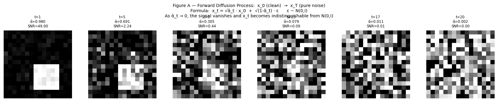
Forward process (easy, no learning): Take a real image. Add a tiny bit of Gaussian noise. Repeat $T$ times. After $T$ steps the image is indistinguishable from pure static.
-
Reverse process (hard, learned): Train a neural network to undo one step of noise at a time. At generation time, start from pure static and denoise step by step until a crisp image emerges.
The mathematical trick that makes this practical is that we can jump to any noise level in one shot — no need to simulate every intermediate step during training.
Chapter 1 — The Noise Schedule
We destroy an image gradually over $T$ timesteps. At each step $t$ we inject noise controlled by a variance parameter $\beta_t$. From $\beta$ we derive two useful quantities:
| Symbol | Definition | Meaning |
|---|---|---|
| $\beta_t$ | chosen per schedule | variance of noise added at step $t$ |
| $\alpha_t$ | $1 - \beta_t$ | fraction of signal kept at step $t$ |
| $\bar{\alpha}_t$ | $\prod_{s=1}^{t} \alpha_s$ | cumulative signal fraction from step 1 to $t$ |
$\bar{\alpha}_t$ is the key number. When $\bar{\alpha}_t \approx 0$ the original image is gone entirely.
T = 20  # timesteps (paper uses 1000; we use 20 for speed)

betas     = torch.linspace(0.02, 0.50, T)       # linear schedule
alphas    = 1.0 - betas                          # signal kept per step
alpha_bar = torch.cumprod(alphas, dim=0)         # cumulative signal

# Precompute the coefficients we'll reuse everywhere
sqrt_alpha_bar           = torch.sqrt(alpha_bar)
sqrt_one_minus_alpha_bar = torch.sqrt(1.0 - alpha_bar)
With this aggressive linear schedule ($\beta$ from 0.02 to 0.50), $\bar{\alpha}_{20} \approx 0.0016$ — only 0.16% of the original signal survives at the final step.
Production note: The original DDPM paper uses $\beta \in [10^{-4},\ 0.02]$ with $T=1000$. Improved DDPM introduced a cosine schedule. Both reach $\bar{\alpha}_T \approx 0$, just via different paths.
Chapter 2 — Synthetic Data
To keep things dependency-free, we generate our own training set: random filled circles and squares on a 16×16 grid.
IMG_SIZE = 16

def make_circle(size=IMG_SIZE):
    img = np.zeros((size, size), dtype=np.float32)
    cx = np.random.uniform(size * 0.3, size * 0.7)
    cy = np.random.uniform(size * 0.3, size * 0.7)
    r  = np.random.uniform(size * 0.2, size * 0.35)
    gy, gx = np.mgrid[0:size, 0:size]
    mask = (gx - cx)**2 + (gy - cy)**2 <= r**2
    img[mask] = 1.0
    return img * 2.0 - 1.0  # normalize to [-1, +1]
Why normalize to $[-1,\, +1]$? The forward process ends at pure Gaussian noise $\mathcal{N}(0, I)$, which is centered at zero. If our clean images lived in $[0, 1]$ the data and noise distributions would sit on different scales, making the reverse process harder to learn. Centering on zero aligns them.
Chapter 3 — The Model: $\varepsilon_\theta(x_t, t)$
The network’s job is straightforward: given a noisy image $x_t$ and the timestep $t$, predict the noise $\varepsilon$ that was mixed in. We use a small MLP with one-hot timestep encoding.
class NoisePredictorMLP(nn.Module):
    def __init__(self):
        super().__init__()
        self.net = nn.Sequential(
            nn.Linear(IMG_DIM + T, 256), nn.GELU(),  # input projection
            nn.Linear(256, 256),         nn.GELU(),  # hidden layer
            nn.Linear(256, IMG_DIM),                  # output: predicted noise
        )

    def forward(self, x_t, t):
        t_emb = F.one_hot(t, num_classes=T).float()  # (B, T)
        inp   = torch.cat([x_t, t_emb], dim=1)       # (B, IMG_DIM + T)
        return self.net(inp)
A few design choices worth noting:
- One-hot timestep encoding is transparent and efficient when $T$ is small. Production models with $T=1000$ use sinusoidal embeddings instead to avoid a 1000-dim sparse vector.
- Concatenation over addition keeps the image and time signals independent — the first 256 dims are always “image,” the last $T$ dims are always “time.”
- GELU over ReLU avoids ReLU’s hard zero-cutoff, which creates gradient discontinuities near zero — a region noise predictions visit often.
Chapter 4 — The Forward Process: $q(x_t \mid x_0)$
Each step of the Markov chain adds noise:
\[x_t = \sqrt{\alpha_t} \cdot x_{t-1} + \sqrt{1 - \alpha_t} \cdot \varepsilon\]But here’s the key insight — we can skip straight to any timestep with a closed-form expression:
\[\boxed{x_t = \sqrt{\bar{\alpha}_t} \cdot x_0 + \sqrt{1 - \bar{\alpha}_t} \cdot \varepsilon,} \qquad \varepsilon \sim \mathcal{N}(0, I)\]The signal coefficient $\sqrt{\bar{\alpha}_t}$ shrinks toward zero while the noise coefficient $\sqrt{1 - \bar{\alpha}_t}$ grows toward one. At $t = T$ the image is pure noise.
Show proof
Proof by induction
This result isn’t magic — it falls out of one key property of Gaussian random variables: if $A \sim \mathcal{N}(0, \sigma_1^2)$ and $B \sim \mathcal{N}(0, \sigma_2^2)$ are independent, then $A + B \sim \mathcal{N}(0,\, \sigma_1^2 + \sigma_2^2)$. Let’s prove the closed form step by step.
Setup. Each forward step is defined as:
\[x_t = \sqrt{\alpha_t} \cdot x_{t-1} + \sqrt{1 - \alpha_t} \cdot \varepsilon_t, \qquad \varepsilon_t \sim \mathcal{N}(0, I), \qquad \alpha_t = 1 - \beta_t\]We want to show that $x_t$ can be written purely in terms of $x_0$ and a single noise draw.
Base case ($t = 1$):
\[x_1 = \sqrt{\alpha_1} \cdot x_0 + \sqrt{1 - \alpha_1} \cdot \varepsilon_1\]Since $\bar{\alpha}_1 = \alpha_1$, this is already in the target form: $x_1 = \sqrt{\bar{\alpha}_1} \cdot x_0 + \sqrt{1 - \bar{\alpha}_1} \cdot \varepsilon_1$. ✓
Inductive step. Assume the claim holds at step $t-1$:
\[x_{t-1} = \sqrt{\bar{\alpha}_{t-1}} \cdot x_0 + \sqrt{1 - \bar{\alpha}_{t-1}} \cdot \bar{\varepsilon}_{t-1}, \qquad \bar{\varepsilon}_{t-1} \sim \mathcal{N}(0, I)\]Now apply one more forward step:
\[x_t = \sqrt{\alpha_t} \cdot x_{t-1} + \sqrt{1 - \alpha_t} \cdot \varepsilon_t\]Substitute the inductive hypothesis for $x_{t-1}$:
\[x_t = \sqrt{\alpha_t} \cdot \left[\sqrt{\bar{\alpha}_{t-1}} \cdot x_0 + \sqrt{1 - \bar{\alpha}_{t-1}} \cdot \bar{\varepsilon}_{t-1}\right] + \sqrt{1 - \alpha_t} \cdot \varepsilon_t\]Distribute $\sqrt{\alpha_t}$:
\[x_t = \sqrt{\alpha_t \bar{\alpha}_{t-1}} \cdot x_0 \;+\; \sqrt{\alpha_t(1 - \bar{\alpha}_{t-1})} \cdot \bar{\varepsilon}_{t-1} \;+\; \sqrt{1 - \alpha_t} \cdot \varepsilon_t\]The first term simplifies immediately since $\alpha_t \cdot \bar{\alpha}_{t-1} = \bar{\alpha}_t$ by definition of the cumulative product:
\[x_t = \sqrt{\bar{\alpha}_t} \cdot x_0 \;+\; \underbrace{\sqrt{\alpha_t(1 - \bar{\alpha}_{t-1})} \cdot \bar{\varepsilon}_{t-1} + \sqrt{1 - \alpha_t} \cdot \varepsilon_t}_{\text{two independent Gaussians — combine them}}\]Since $\bar{\varepsilon}_{t-1}$ and $\varepsilon_t$ are independent, their weighted sum is Gaussian with variance equal to the sum of their scaled variances:
\[\text{Var} = \alpha_t(1 - \bar{\alpha}_{t-1}) + (1 - \alpha_t)\]Expanding:
\[= \alpha_t - \alpha_t \bar{\alpha}_{t-1} + 1 - \alpha_t = 1 - \alpha_t \bar{\alpha}_{t-1} = 1 - \bar{\alpha}_t\]So the two noise terms collapse into a single Gaussian:
\[\sqrt{\alpha_t(1 - \bar{\alpha}_{t-1})} \cdot \bar{\varepsilon}_{t-1} + \sqrt{1 - \alpha_t} \cdot \varepsilon_t \;=\; \sqrt{1 - \bar{\alpha}_t} \cdot \varepsilon, \qquad \varepsilon \sim \mathcal{N}(0, I)\]Putting it together:
\[\boxed{x_t = \sqrt{\bar{\alpha}_t} \cdot x_0 + \sqrt{1 - \bar{\alpha}_t} \cdot \varepsilon} \qquad \blacksquare\]This is why torch.cumprod is all we need to precompute the schedule — the entire multi-step chain reduces to one multiplication and one addition.
def q_sample(x0, t, noise):
    """Corrupt x_0 directly to noise level t (no sequential simulation)."""
    sa  = sqrt_alpha_bar[t].unsqueeze(1)            # (B, 1)
    soa = sqrt_one_minus_alpha_bar[t].unsqueeze(1)  # (B, 1)
    return sa * x0 + soa * noise                    # (B, IMG_DIM)
This is what makes DDPM training efficient — each batch element can jump to a random noise level in $O(1)$.
Chapter 5 — Training
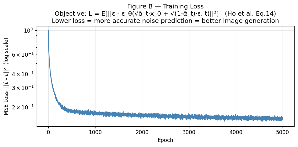
The training objective is beautifully simple. It comes from a simplification of the variational lower bound (ELBO), as shown in Ho et al. (Eq. 14):
\[\mathcal{L} = \mathbb{E}\!\left[\left\|\varepsilon - \varepsilon_\theta(x_t, t)\right\|^2\right]\]In plain English: sample a random timestep, corrupt the image, ask the network to predict the noise, and minimize the mean squared error.
for epoch in range(EPOCHS):
    for x0 in dataloader:
        x0 = x0.to(device)
        B  = x0.shape[0]

        t     = torch.randint(0, T, (B,), device=device)  # random timestep
        noise = torch.randn_like(x0)                       # ε ~ N(0, I)
        x_t   = q_sample(x0, t, noise)                     # corrupt

        eps_pred = model(x_t, t)                            # predict noise
        loss     = F.mse_loss(eps_pred, noise)              # compare

        optimizer.zero_grad()
        loss.backward()
        optimizer.step()
Sampling $t$ uniformly ensures every noise level gets equal training attention — both the near-clean images (small $t$) and the nearly destroyed ones (large $t$).
Chapter 6 — Sampling: The Reverse Process
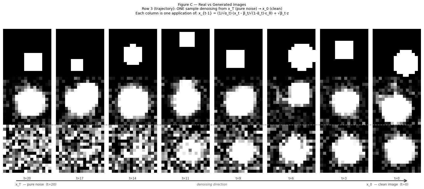
This is where the magic happens. Starting from pure noise $x_T \sim \mathcal{N}(0, I)$, we denoise one step at a time.
The reverse step formula is derived by applying Bayes’ theorem to the forward process, substituting our noise prediction, and simplifying:
\[x_{t-1} = \frac{1}{\sqrt{\alpha_t}} \left[x_t - \frac{\beta_t}{\sqrt{1 - \bar{\alpha}_t}} \cdot \varepsilon_\theta(x_t, t)\right] + \sqrt{\beta_t} \cdot z\]where $z \sim \mathcal{N}(0, I)$ for $t > 0$ and $z = 0$ at the final step.
Show proof
Derivation of the reverse step
The key insight is that while the reverse marginal $p(x_{t-1} \mid x_t)$ is intractable, the posterior conditioned on $x_0$ is not.
Step 1: Apply Bayes’ theorem.
\[q(x_{t-1} \mid x_t, x_0) = \frac{q(x_t \mid x_{t-1})\, q(x_{t-1} \mid x_0)}{q(x_t \mid x_0)}\]The denominator $q(x_t \mid x_0)$ is just a normalising constant with respect to $x_{t-1}$, so we only need to work with the numerator.
Step 2: Write the two Gaussian factors.
From the one-step forward kernel:
\[q(x_t \mid x_{t-1}) = \mathcal{N}\!\left(x_t;\; \sqrt{\alpha_t}\, x_{t-1},\; \beta_t I\right)\]From the closed-form forward process (Chapter 4):
\[q(x_{t-1} \mid x_0) = \mathcal{N}\!\left(x_{t-1};\; \sqrt{\bar{\alpha}_{t-1}}\, x_0,\; (1-\bar{\alpha}_{t-1}) I\right)\]Step 3: Complete the square to find the posterior mean and variance.
Taking the log of the numerator and collecting terms in $x_{t-1}$:
\[\log q(x_{t-1} \mid x_t, x_0) \propto -\frac{(x_t - \sqrt{\alpha_t}\, x_{t-1})^2}{2\beta_t} - \frac{(x_{t-1} - \sqrt{\bar{\alpha}_{t-1}}\, x_0)^2}{2(1-\bar{\alpha}_{t-1})}\]Expanding and grouping by powers of $x_{t-1}$, the coefficient of $x_{t-1}^2$ gives the posterior variance:
\[\frac{1}{\tilde{\beta}_t} = \frac{\alpha_t}{\beta_t} + \frac{1}{1-\bar{\alpha}_{t-1}} = \frac{\alpha_t(1-\bar{\alpha}_{t-1}) + \beta_t}{\beta_t(1-\bar{\alpha}_{t-1})}\]The numerator simplifies using $\beta_t = 1 - \alpha_t$:
\[\alpha_t(1-\bar{\alpha}_{t-1}) + \beta_t = \alpha_t - \bar{\alpha}_t + 1 - \alpha_t = 1 - \bar{\alpha}_t\]So:
\[\tilde{\beta}_t = \frac{\beta_t(1 - \bar{\alpha}_{t-1})}{1 - \bar{\alpha}_t}\]The linear coefficient in $x_{t-1}$ gives the posterior mean:
\[\tilde{\mu}_t(x_t, x_0) = \tilde{\beta}_t\!\left(\frac{\sqrt{\alpha_t}}{\beta_t}\, x_t + \frac{\sqrt{\bar{\alpha}_{t-1}}}{1-\bar{\alpha}_{t-1}}\, x_0\right) = \frac{\sqrt{\alpha_t}(1-\bar{\alpha}_{t-1})}{1-\bar{\alpha}_t}\, x_t + \frac{\sqrt{\bar{\alpha}_{t-1}}\,\beta_t}{1-\bar{\alpha}_t}\, x_0\]So the posterior is:
\[q(x_{t-1} \mid x_t, x_0) = \mathcal{N}\!\left(x_{t-1};\; \tilde{\mu}_t(x_t, x_0),\; \tilde{\beta}_t I\right)\]Step 4: Eliminate $x_0$ using the noise prediction.
We cannot condition on the unknown $x_0$ at sampling time. Inverting the Chapter 4 forward formula gives:
\[x_0 = \frac{x_t - \sqrt{1-\bar{\alpha}_t}\;\varepsilon_\theta(x_t, t)}{\sqrt{\bar{\alpha}_t}}\]Substitute this into the posterior mean from Step 3:
\[\tilde{\mu}_t = \frac{\sqrt{\alpha_t}(1-\bar{\alpha}_{t-1})}{1-\bar{\alpha}_t}\, x_t + \frac{\sqrt{\bar{\alpha}_{t-1}}\,\beta_t}{1-\bar{\alpha}_t} \cdot \frac{x_t - \sqrt{1-\bar{\alpha}_t}\;\varepsilon_\theta}{\sqrt{\bar{\alpha}_t}}\]Use $\sqrt{\bar{\alpha}_{t-1}}/\sqrt{\bar{\alpha}_t} = 1/\sqrt{\alpha_t}$ to simplify the second term:
\[\tilde{\mu}_t = \frac{\sqrt{\alpha_t}(1-\bar{\alpha}_{t-1})}{1-\bar{\alpha}_t}\, x_t + \frac{\beta_t}{(1-\bar{\alpha}_t)\sqrt{\alpha_t}}\!\left(x_t - \sqrt{1-\bar{\alpha}_t}\;\varepsilon_\theta\right)\]Factor out $\dfrac{1}{(1-\bar{\alpha}_t)\sqrt{\alpha_t}}$ from both $x_t$ terms:
\[\tilde{\mu}_t = \frac{x_t}{(1-\bar{\alpha}_t)\sqrt{\alpha_t}}\!\left[\alpha_t(1-\bar{\alpha}_{t-1}) + \beta_t\right] - \frac{\beta_t}{\sqrt{\alpha_t}\sqrt{1-\bar{\alpha}_t}}\;\varepsilon_\theta\]The bracket $\alpha_t(1-\bar{\alpha}_{t-1}) + \beta_t = 1-\bar{\alpha}_t$ (shown in Step 3), so the $x_t$ coefficient collapses:
\[\tilde{\mu}_t = \frac{1}{\sqrt{\alpha_t}}\!\left(x_t - \frac{\beta_t}{\sqrt{1-\bar{\alpha}_t}}\;\varepsilon_\theta(x_t,t)\right)\]Step 5: Draw the sample.
Sampling from $\mathcal{N}(\tilde{\mu}_t, \tilde{\beta}_t I)$ with the reparameterisation trick, and using $\sigma_t = \sqrt{\beta_t}$ as the noise scale:
\[\boxed{x_{t-1} = \frac{1}{\sqrt{\alpha_t}}\!\left(x_t - \frac{\beta_t}{\sqrt{1-\bar{\alpha}_t}}\;\varepsilon_\theta(x_t,t)\right) + \sqrt{\beta_t}\cdot z} \qquad \blacksquare\]@torch.no_grad()
def p_sample(model, x_t, t_scalar):
"""One reverse step: x_t → x_{t-1}."""
B = x_t.shape[0]
t_batch = torch.full((B,), t_scalar, device=device, dtype=torch.long)
eps_pred = model(x_t, t_batch)
coeff1 = 1.0 / sqrt_alphas[t_scalar]
coeff2 = betas[t_scalar] / sqrt_one_minus_alpha_bar[t_scalar]
mean = coeff1 * (x_t - coeff2 * eps_pred)
if t_scalar == 0:
return mean # deterministic final step
else:
z = torch.randn_like(x_t)
return mean + sqrt_betas[t_scalar] * z
Why add noise at every step except the last? The stochasticity is what gives the model its generative diversity. Two runs from different starting noise produce different images. At $t = 0$ we want the clean result, so we drop the noise term.
To generate a full image, we just loop from $T-1$ down to 0:
@torch.no_grad()
def p_sample_loop(model, n_samples=8):
    x = torch.randn(n_samples, IMG_DIM, device=device)  # start from noise
    for t in reversed(range(T)):
        x = p_sample(model, x, t)
    return x
Putting It All Together
Here’s the full algorithm at a glance:
1. Forward — destroy the image in one shot
\[x_t = \sqrt{\bar{\alpha}_t} \cdot x_0 + \sqrt{1-\bar{\alpha}_t} \cdot \varepsilon\]2. Train — teach the network to predict noise
\[\mathcal{L} = \mathbb{E}\!\left[\left\|\varepsilon - \varepsilon_\theta(x_t, t)\right\|^2\right]\]3. Sample — denoise step by step from pure noise
\[x_{t-1} = \frac{1}{\sqrt{\alpha_t}} \left(x_t - \frac{\beta_t}{\sqrt{1-\bar{\alpha}_t}} \cdot \varepsilon_\theta(x_t, t)\right) + \sqrt{\beta_t} \cdot z\]With 4,096 tiny training images, a 3-layer MLP, and 20 diffusion steps, the model learns to generate recognizable circles and squares in a few minutes on a laptop.
Where to Go from Here
This minimal implementation keeps every moving part visible. To scale up toward production-quality generation:
- Replace the MLP with a U-Net to exploit spatial structure via skip connections.
- Use sinusoidal time embeddings when $T$ grows to 1000+.
- Try DDIM for deterministic, fewer-step sampling at inference time.
- Add classifier-free guidance to condition generation on class labels or text prompts.
- Explore score-based models — the continuous-time generalization of this framework.
The full runnable script (one file, zero external datasets) is available in microdiffusion.py.
Authors
Harsh Agarwal — MS in Robotics, Carnegie Mellon University. GitHub
Claude (Anthropic) — AI assistant. This post was written in collaboration with Claude, which helped structure the derivations, write the proofs, and format the mathematical notation.
Reference: Ho, Jain & Abbeel, “Denoising Diffusion Probabilistic Models,” NeurIPS 2020. arXiv:2006.11239