A description of the depth network that we worked on in Adelaide!

In the previous post we established the idea that how can we estimate the pose from src to target in an unsupervised manner, if we are given a reasonable depth map and decent depth features of the target image.

In this post we would try focussing on getting a depth network which could be used for this task.

Ravi Garg in his work had used a network architecture, for single view depth estimation, trained on KITTI dataset using stereo pairs. Please look here for visualising Ravi’s network. On using this architecture as it is, we were not able to train it reasonably for NYUDv2. Most of the papers currently except that of Eigen’s primarily focus on outdoor datasets like KITTI, CityScapes and so on. Training for pose and depth on NYUDv2 seems like a challenge. Why? My key observations are:

• Diversity : It might be easy to learn outdoor data sets, as there is less diversity. As in all the roads, more or less look the same. If you are travelling through the city, you may not expect that the scene changes so drastically that the network feels lost. This is one point pointed out by even Elon Musk in his TED! On the other hand just imagine you learned the structure of a study room, now you go to a different room, the structure can be so different that you get confused thinking if it is even a study room at all! And NYUDv2 on keenly observing has too many images but the variations between them aren’t much.

• Data Capture : The NYUDv2 data has been recorded by a person moving around with a handheld camera. In contrary to other datasets that have been recorded on car or robots. So the kind of complexity and the random nature of the dataset make it challenging to work with.

And we wanted to work on NYUDv2. So, as Ravi’s network (it is kind of a tradition that our nomenclature just add’s the name of the people who have made it, HuangYing’s Layer, Ravi’s network :P) did not work on NYUDv2, I and Saroj started designing a depth network. Saroj was working with Eigen’s network for the some other projects, and felt we could design an architecture which could be simpler and easy to train as compared to Eigen with equivalent performance. So taking insights from HuangYing and Saroj, I prepared a U-Net kind of an architecture for Depth estimation in NYUDv2 using Eigen’s loss. Other losses that I tweaked with were L2, L2 with smoothness regularization. Eventually we decided to go on with Eigen’s loss.

Eigen’s Loss

In NIPS 2014 Depth Map Prediction from a Single Image using a Multi-Scale Deep Network by Eigen et al. proposed a scale invariant error. The following was the loss function proposed:

\[D(y,y^*) = \frac{1}{2n}\sum_{i=1}^{n}(\log(y_i) - \log(y^*_i) + \alpha(y,y^*))^2\]

where \(\alpha(y,y^*) = \sum_i(\log(y^*_i) - \log(y_i))\)

The equivalent form of the above loss function can be thought of as:

\[D(y,y^*) = \frac{1}{2n^2}\sum_{i,j}((\log y_i - \log y_j)-(\log y^*_i -\log y^*_j))^2\]

Quoting lines from the paper:

The above formulation expresses the error by comparing relationships between pairs of pixels i, j in the output: to have low error, each pair of pixels in the prediction must differ in depth by an amount similar to that of the corresponding pair in the ground truth.

Makes sense? Isn’t it? This loss becomes scale-invariant in nature! Magical properties of $\log$ you see ;)

Now, using \(d_i = \log y_i - \log y^*_i\) to be the difference between the prediction and the ground truth at pixel \(i\) we can write:

\(D(y,y^*) = \frac{1}{2n^2}\sum_{i,j}(d_i - d_j)^2\) \(\implies D(y,y^*) = \frac{1}{2n^2}\sum_{i,j}(d^2_i + d^2_j - 2d_id_j)\) \(\implies D(y,y^*) = \frac{1}{2n^2}\sum_{i}\sum_{j}(d^2_i + d^2_j - 2d_id_j)\) \(\implies D(y,y^*) = \frac{1}{2n^2}\sum_{i}(nd^2_i + \sum_jd^2_j - \sum_j2d_id_j)\) \(\implies D(y,y^*) = \frac{1}{2n^2}(n\sum_{i}d^2_i + n\sum_jd^2_j - \sum_i\sum_j2d_id_j)\) \(\implies D(y,y^*) = \frac{2n}{2n^2}\sum_i d^2_i - \frac{1}{n^2}\sum_{i,j}d_id_j\) \(\implies D(y,y^*) = \frac{1}{n}\sum_i d^2_i - \frac{1}{n^2}(\sum_i d_i)^2\)

Again, as the paper says:

The last formulation relates the error metric to the original $l_2$ error, but with an additional term, $-\frac{1}{n^2}\sum_{i,j}d_id_j$ , that credits mistakes if they are in the same direction and penalizes them if they oppose. Thus, an imperfect prediction will have lower error when its mistakes are consistent with one another. The final equation rewrites the formulation so as to perform the operation in a linear-time computation.

The actual training loss that has been used for training is as follows:

\[L(y,y^*) = \frac{1}{n}\sum_i d^2_i - \frac{\lambda}{n^2}(\sum_i d_i)2\]

$\lambda$ is our weight for the scale invariant term. Using $\lambda = 0$ we essentially get L2 loss and putting $\lambda = 1$ makes it completely scale invariant. We in our experiments would be using $\lambda = 0.5$

So we have established the Eigen’s loss and why did we decide to go for it!

The project can be found at _______ (put the link here)

Results

To give you a tentative idea I am posting some depth maps that we had obtained.

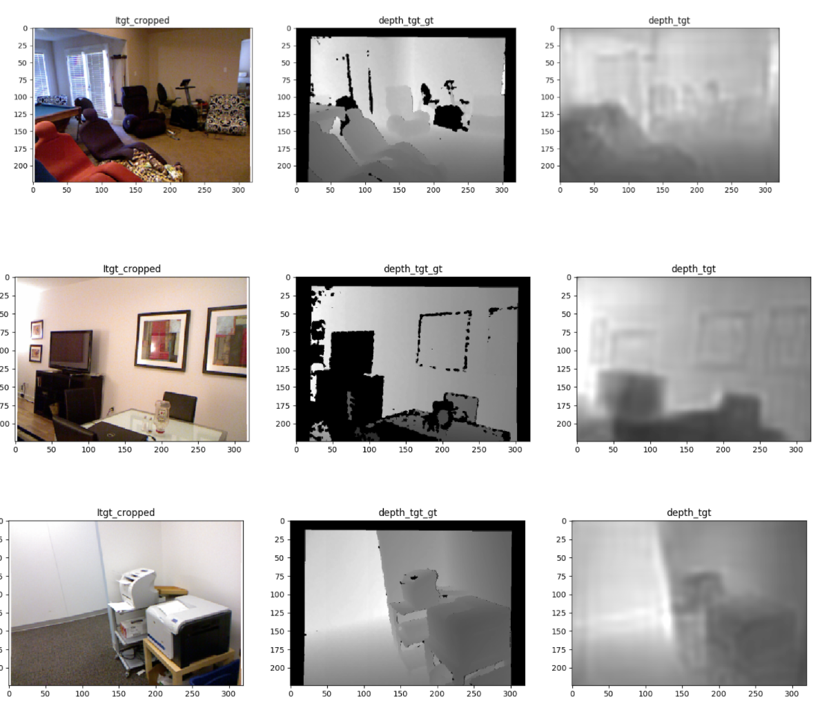
I am trying to generate the results in a comprehensive manner, I need to repeat some set of experiments and then get them. I seem to have left them in Adelaide :P. I will regenerate the results and post them as soon as I get some free time :)

Conclusion

In essence, we have made a depth network whose features can be tapped in from a suitable point for pose as well as depth estimation.

Well, here my internship ended and the next set of experiments are being carried out by Ravi Garg at University of Adelaide.

Cheers,

Harsh Agarwal