After my sophomore year I started working on sketches! Sketches are very different from images. Let’s take an example to understand this.

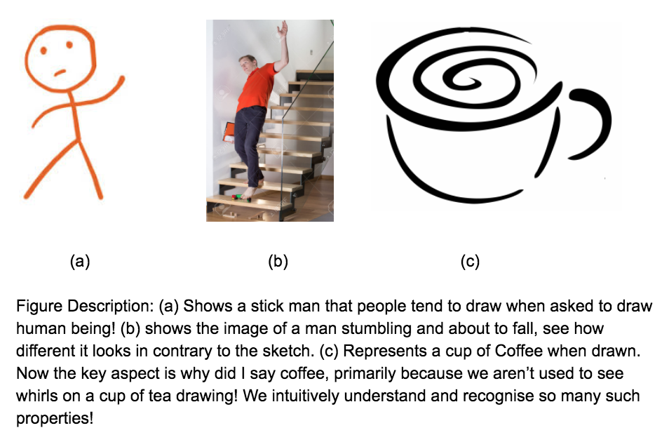
The last image has been taken from Eye_of_the_Dragon: Exploring Discriminatively Minimalist Sketch-based Abstractions for Object Categories

Even though sketches are so different, yet humans are able to understand skecthes pretty intuitively and easily. There are some characteristic features that are involved with a particular type of sketches. we somhow have been trained to recognise such features given the enormous data that we have been fed with since our childhood! Can we expect a neural network to do that job?

This was my project at IISc Bangalore, which I ended up getting after my quest of augmenting anything that we think about. You can read about that …….

The idea was to understand sketches in detail. So we started working on this project! How to approach this problem? The basic idea is:

Images have too much of information and sketches have too sparse information. So we need to somehow decrease the information in the images and increase the information in a skecth to come to a mid level representation that can be used to compare these two entities!

Simple enough! But how do we do it? We don’t really have a dataset dedicated to sketch segmentation and annotation! So we started collecting dataset at the same time thinking about alternatives.

After several failed attempts we finally decided to simply sketchify the images in PASCAL VOC Dataset. So in essence we brought image to the sketch embedding space. Now we can train this network on these transformed images. So we have:

• ‘skecthified’ images
• parts correponding to these images so in essence we have parts form sketchified images as well!

We finally got substantial data to train our network. Yipee!

Quoting Yoshua Bengio’s answer to “Is fine tuning a pre-trained model equivalent to transfer learning?”:

Yes, if the data on which the model is fine-tuned is of a different nature from the original data used to pre-train the model. It is a form of transfer learning, and it has worked extremely well in many object classification tasks.

This was the “Eureka Moment!” So we started working in this direction. We had to do a couple of things before we could get this check our idea. Primarily:

1. Get a suitable sketch like representation on which we could train the network.
2. Design a network to segment sketches pixel wise in a manner analogous to images.

For the first part we started experimenting with various forms of sketches. Main questions that we had were:

1. What if we ran just canny edge detector and trained the network!
2. Can we add some more detail using part boundary explicitly?
3. Can we design a deep network for sketchifying the images even? Like using DeepContours (PUT THE LINK TO THE PAPER)

For the network, we decided to use a standard network designed for image segmentation to start our experiments. DeepLabV2 (PUT THE LINK)

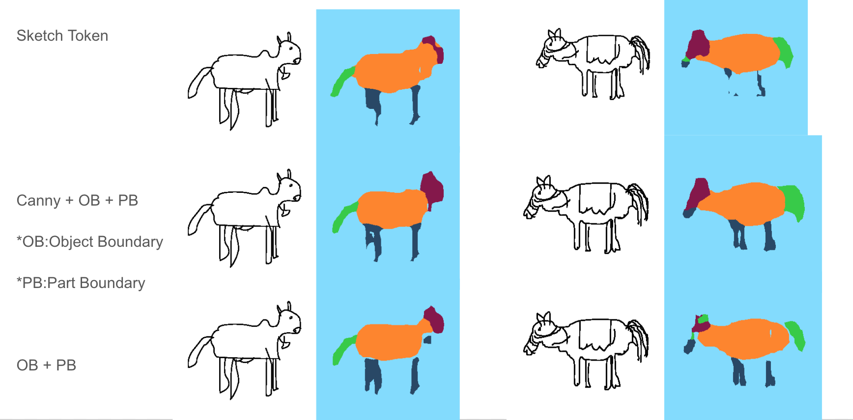
So let’s take up the first question. What representation to choose? Well, we tried training some categories (‘Cows’ and ‘Horses’) with various representation that helped us in qualitatively decide which representations can we go for! wanna have a look? See!

Although the network was trained on cows and horses it performs reasonably on cats even:

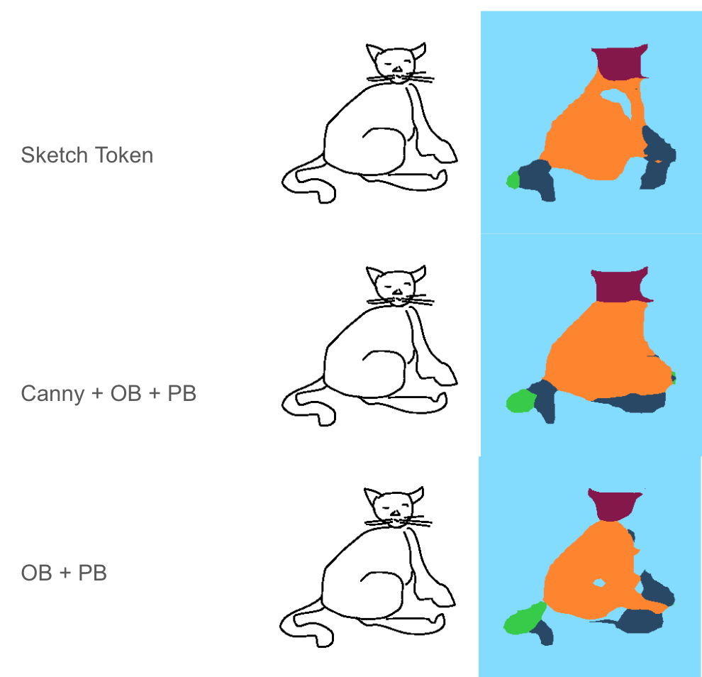
Looking at the above result we decided we would be using OB + PB + Canny and from skecthes in the following manner:

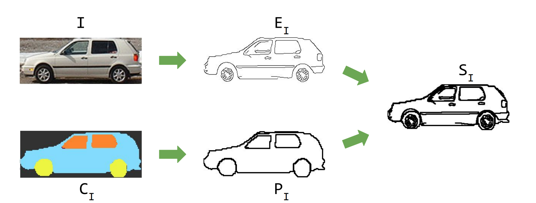
So after preparing the images in the foellowing manner, we had to train this network for various categories.

We slowly and steadily started increasing the number of categories. Possibly bacause of variations in pose and diversity of sketches, the network started getting confused.

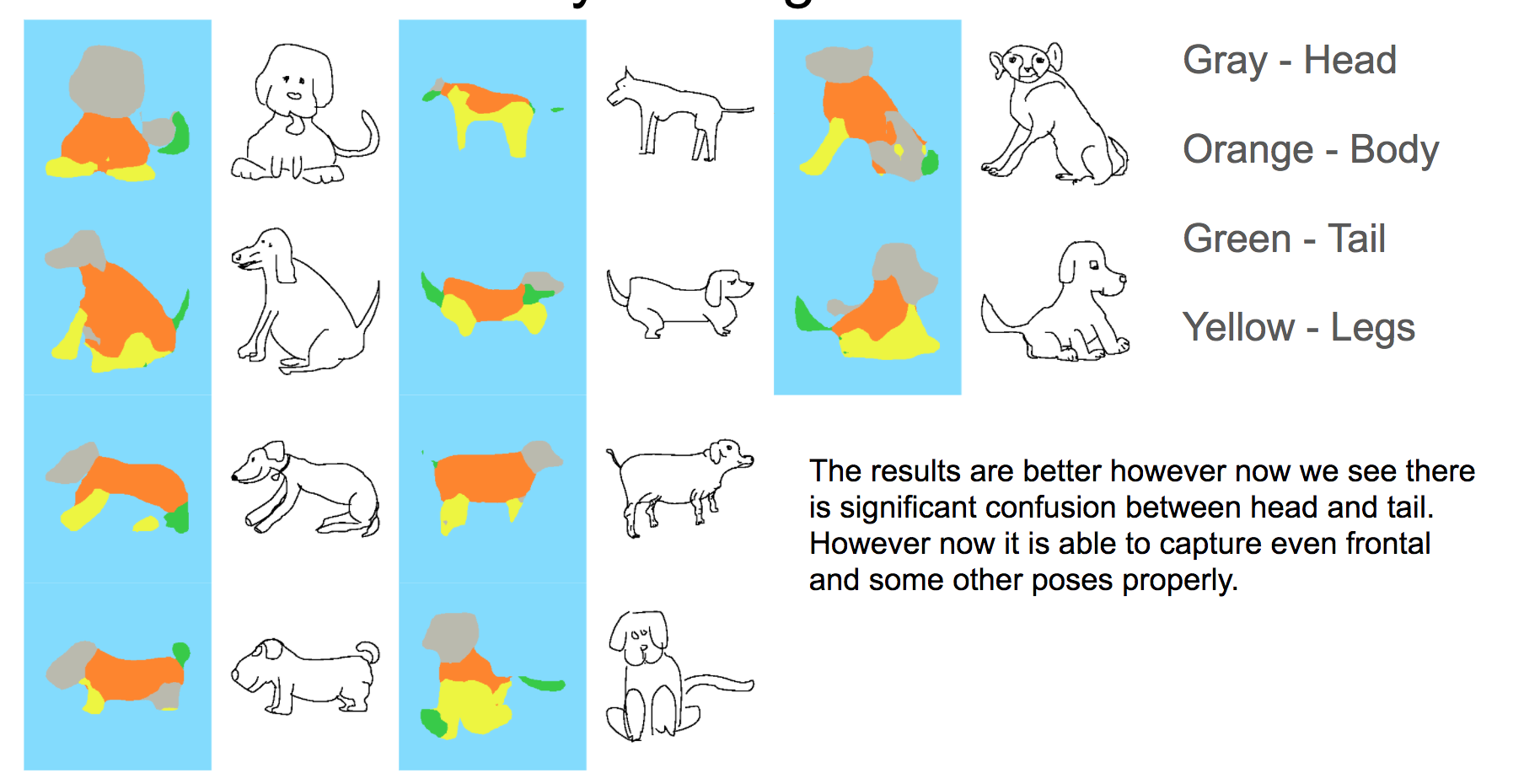
For instance when we trained on ‘cat’,’cow’,’horse’,’sheep’ and dogs’, the following results were obtained!

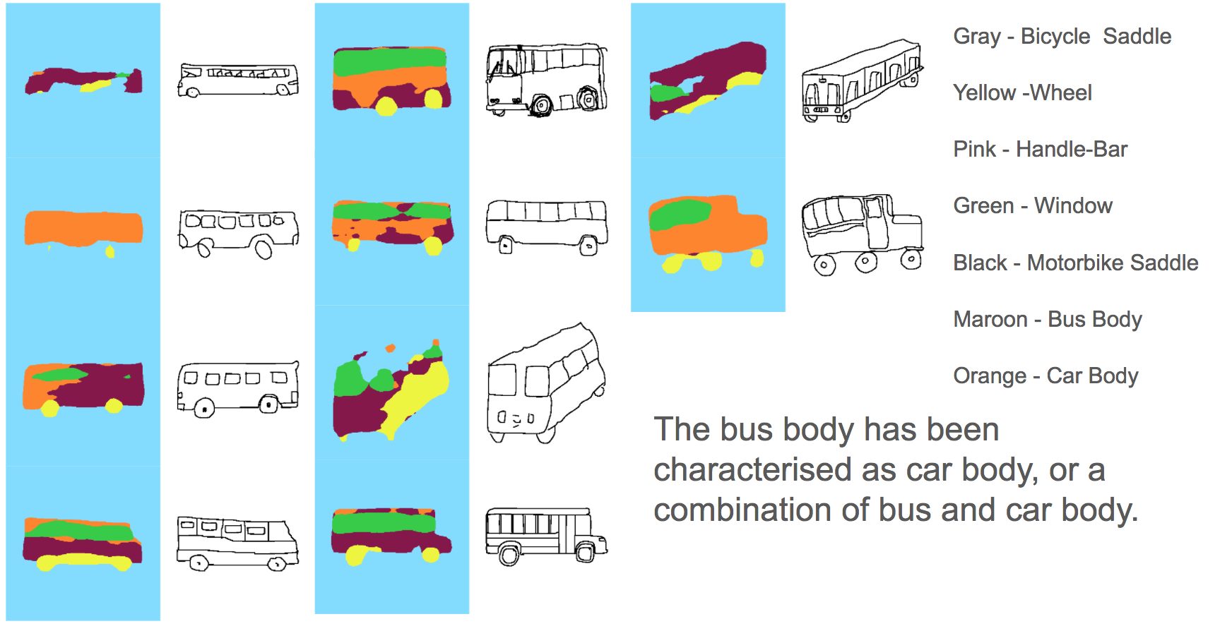
Training the network for Bus, Car, Motorbike, Bicycle gives something like this:

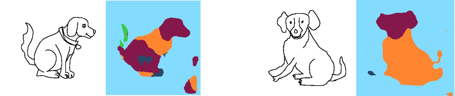
Trying separate categories works very well…See..A network trained only to segment ‘Dogs’:

So what we get from this is, that we need to use a kind of a routing layer to define some routes to segmentation. A schematic version of that is shown here:

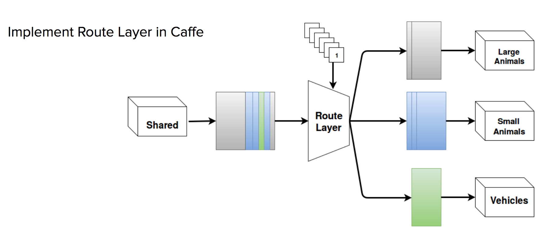
Implementation of this layer has been done by Sahil Manocha(PUT THE LINK). If interested you can look at the details and the code written by him here(PUT THE LINK)

As Sahil was implementing this I realised that if somehow we could place a prior in the network just the way we understand and rectify bad results intuitively. Can we make that happen!

Now we had two options either we could use a CRF, or we could mathematically create a model that in essence did what a CRF did, classical Machine Learning!

I was asked to work on the classical Machine Learning approach. Let’s see!

Implementing a CRF using GMM

The idea was to post process the segmentation that we obtained from the DeepNet. So I tried implementing mathematically something inline to CRF using GMM’s and probability. Let’s have a look the approach.

A very intuitive and precise idea behind CRF’s can be found in Tomasz Malisiewicz’s answer to How are Conditional Random Fields applied to image segmentation?

He states:

CRFs typically involve a local potential and a pairwise potential. The local potential is usually the output of a pixelwise classifier applied to an image. The result is usually not smooth. The pairwise potential favors pixel neighbors which don’t have an image gradient between them to have the same label. Finally an inference algorithm is ran which finds the best setting of labels to pixels.

So we need two things:

1. A measure that tells us a individual part likelihood of a part in a given segmentation.
2. A parwise likelihood of various combination of parts that we have in a particular segmentation.

In addition to we would also be adding the deciation from the avg. connectivity graph. It’s ‘OK’ if you are not able to understand the jargon that I am using. As we go ahead we would be defining all the terms :)

So how do we describe the parts with out a deep net? We need features, classical Machine Learning! Yay!

With some toy experiments we were able to conclude that the following feature vector can completely represent a part.

\[M = \left( \begin{array}{cccc} RelativeArea & RoundedNess & Centroid(x) & Centroid(y) \\ \end{array} \right)\]

where:

\[RelativeArea = AreaOfObject/AreaOfPart \\ Roundedness = Area/(Perimeter)^2 \\ Centroid(x) = x-coordinate of the Centroid \\ Centroid(y) = y-coordinate of the Centroid \\\]

If I can hypothesise this then using Baye’s theorem I can easily say:

\[P(X/Y) = \frac{P(Y/X)P(X)}{P(Y)} \\\]

Let’s try elaborating it a bit: \(P(\hspace{1mm}that\hspace{1mm}a\hspace{1mm}part\hspace{1mm}is\hspace{1mm}a\hspace{1mm}'head'\hspace{1mm}given\hspace{1mm}it\hspace{1mm}has\hspace{1mm}a\hspace{1mm}feature\hspace{1mm}'f1') = \frac{P(the\hspace{1mm}part\hspace{1mm}has\hspace{1mm}a \hspace{2mm}feature\hspace{1mm}'f1'\hspace{1mm}given\hspace{1mm}it\hspace{1mm}is\hspace{1mm}a\hspace{1mm}head)P(it\hspace{1mm}is\hspace{1mm}a\hspace{1mm}head)}{P(it\hspace{1mm}has\hspace{1mm}a\hspace{1mm}feature\hspace{1mm}'f1')}\)

As are pretty sure that the blob that we are trying to work on has the feature that we have calculated the denominator becomes 1. This means that we can say:

\[P(\hspace{1mm}that\hspace{1mm}a\hspace{1mm}part\hspace{1mm}is\hspace{1mm}a\hspace{1mm}'head'\hspace{1mm}given\hspace{1mm}it\hspace{1mm}has\hspace{1mm}a\hspace{1mm}feature\hspace{1mm}'f1') = \frac{P(the\hspace{1mm}part\hspace{1mm}has\hspace{1mm}a \hspace{2mm}feature\hspace{1mm}'f1'\hspace{1mm}given\hspace{1mm}it\hspace{1mm}is\hspace{1mm}a\hspace{1mm}head)P(it\hspace{1mm}is\hspace{1mm}a\hspace{1mm}head)}{1}\] \[\implies P(\hspace{1mm}that\hspace{1mm}a\hspace{1mm}part\hspace{1mm}is\hspace{1mm}a\hspace{1mm}'head'\hspace{1mm}given\hspace{1mm}it\hspace{1mm}has\hspace{1mm}a\hspace{1mm}feature\hspace{1mm}'f1') \propto P(the\hspace{1mm}part\hspace{1mm}has\hspace{1mm}a \hspace{2mm}feature\hspace{1mm}'f1'\hspace{1mm}given\hspace{1mm}it\hspace{1mm}is\hspace{1mm}a\hspace{1mm}head) - (1)\]

We can calculate the RHS of the above equation. How do we do that? Tell me one thing, what are we trying to do when we are minimising the cross entropy loss and training a network? We are trying to get a probability distribution very close to what our training data has. Lemme show you:

\[I(x) = -log(P(x))\]

\(H(x) = E_{x \sim p}[I(x)] = -E_{x \sim p}[log(P(x))]\) Shanon entropy of a distribution is the expected amount of information in an event drawn from that distribution. If x~ Continuous Variable then Shanon Entropy is referred to as differential entropy.

The KL(Kullback-Leibler) divergence is given by:

\[D_{KL}(P||Q) = E_{x \sim p}[\log(\frac{P(x)}{Q(x)})] \implies D_{KL}(P||Q) = E_{x \sim p}[\log(P(x)) - \log(Q(x))]\]

And Cross Entropy is defined as:

\[H(P,Q) = H(P) + D_{KL}(P||Q) \implies H(P,Q) = -E_{x \sim p}[\log(P(x))] + E_{x \sim p}[\log(\frac{P(x)}{Q(x)})] \implies H(P,Q) = -E_{x \sim p}[\log(Q(x))]\]

When we are trying to minimise the cross entropy loss, looking at the first equation we can say that we are trying to minimize the KL-divergence between the probability distributions P and Q. This means that we are trying to get a probability distribution Q which is very similar to P. In essence saying that the amount of self information that we have in Q is equivalent to waht we have in P aka the train set!

No, my idea was to use a Gaussian Mixture Model to approximate the distribution of the desired feature vectors in the train set. Using that probability distribution we would be able to calculate the RHS of equation 1. That would help us in calculating the part wise and pair wise potentials. Adding all such potentials along with the deviation from the average neighbourhood matrix would be used as a measure to caculate which segmentation (with the current labelling) is suitable.

To get the suitability of the segmentation we would be training SVM models. Once we get the uncertain segments, we would try replacing those segments and decreasing the energy! In this way we would be able to correct the segmentation to some extent.

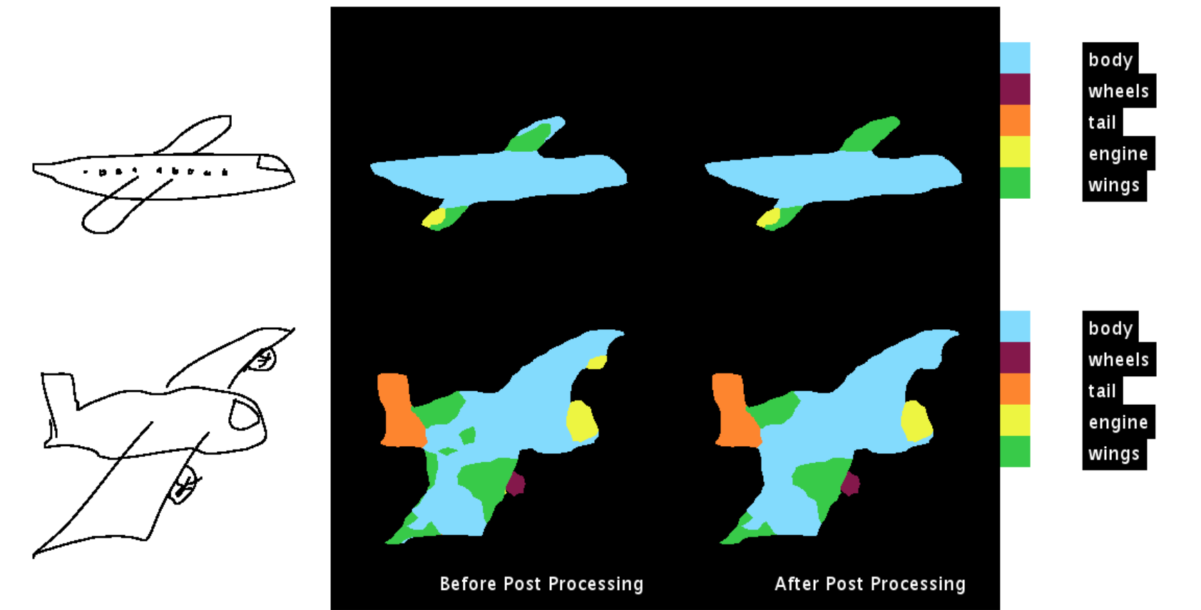
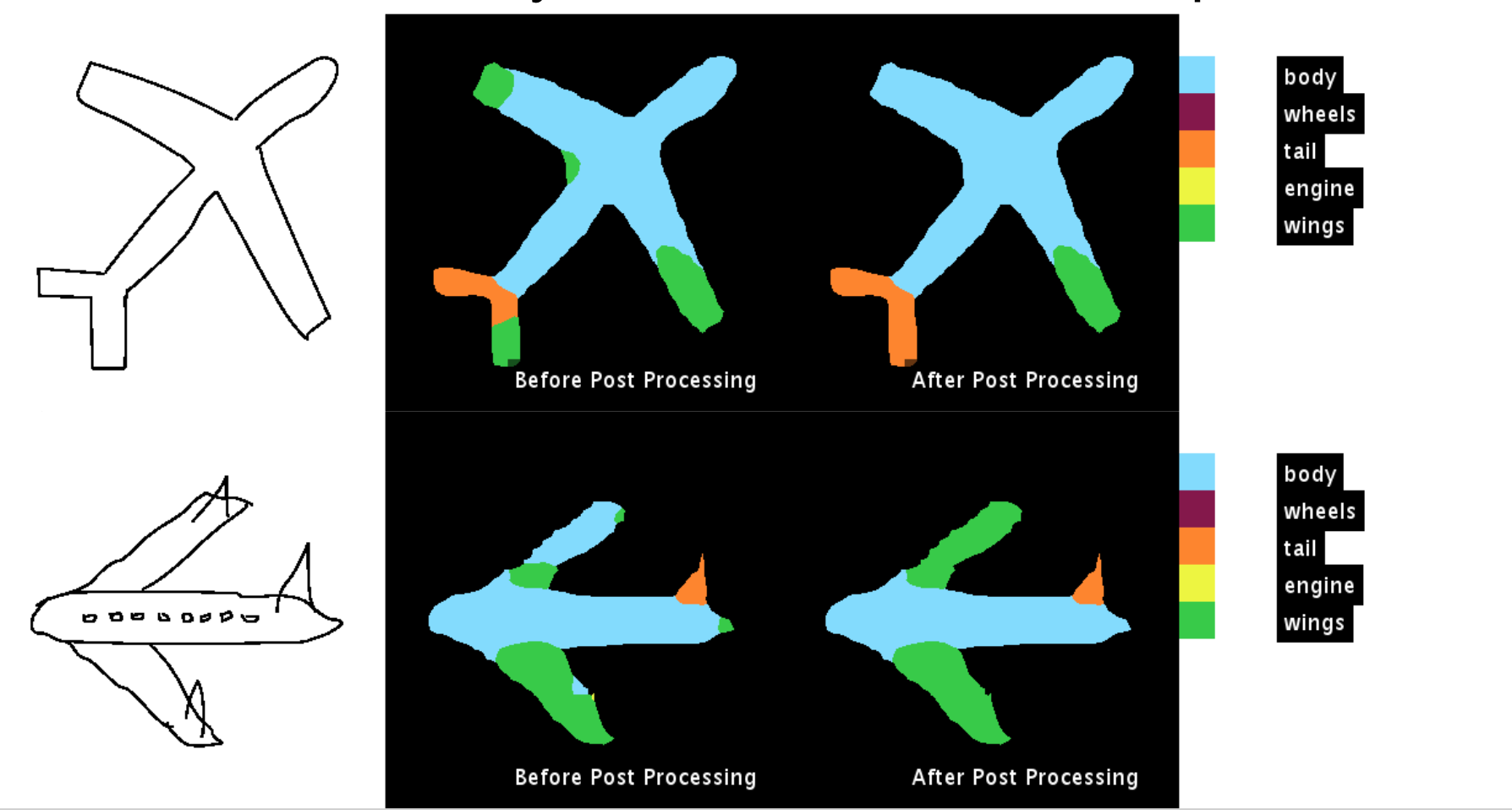
The following are some of the results obtained:

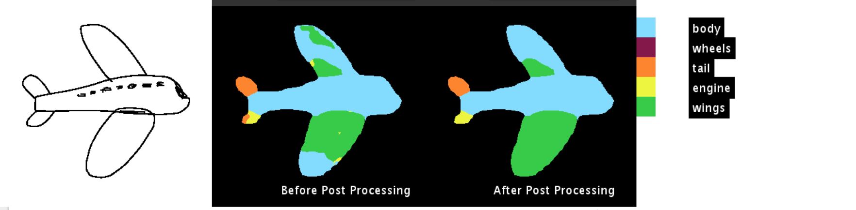
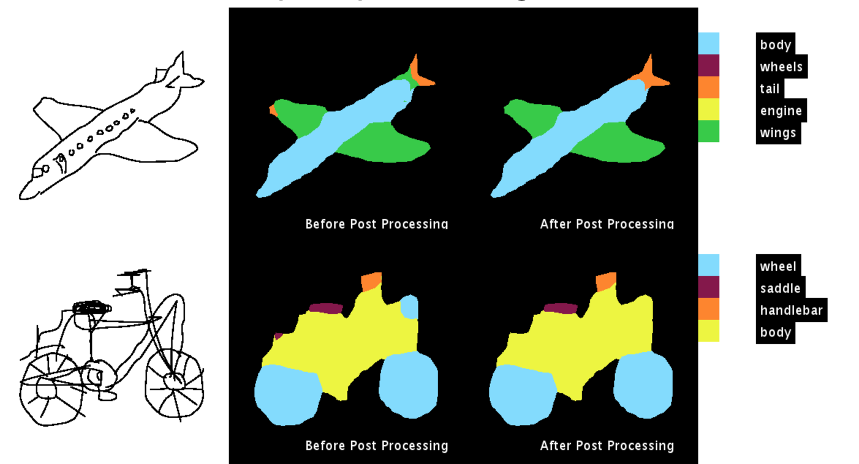
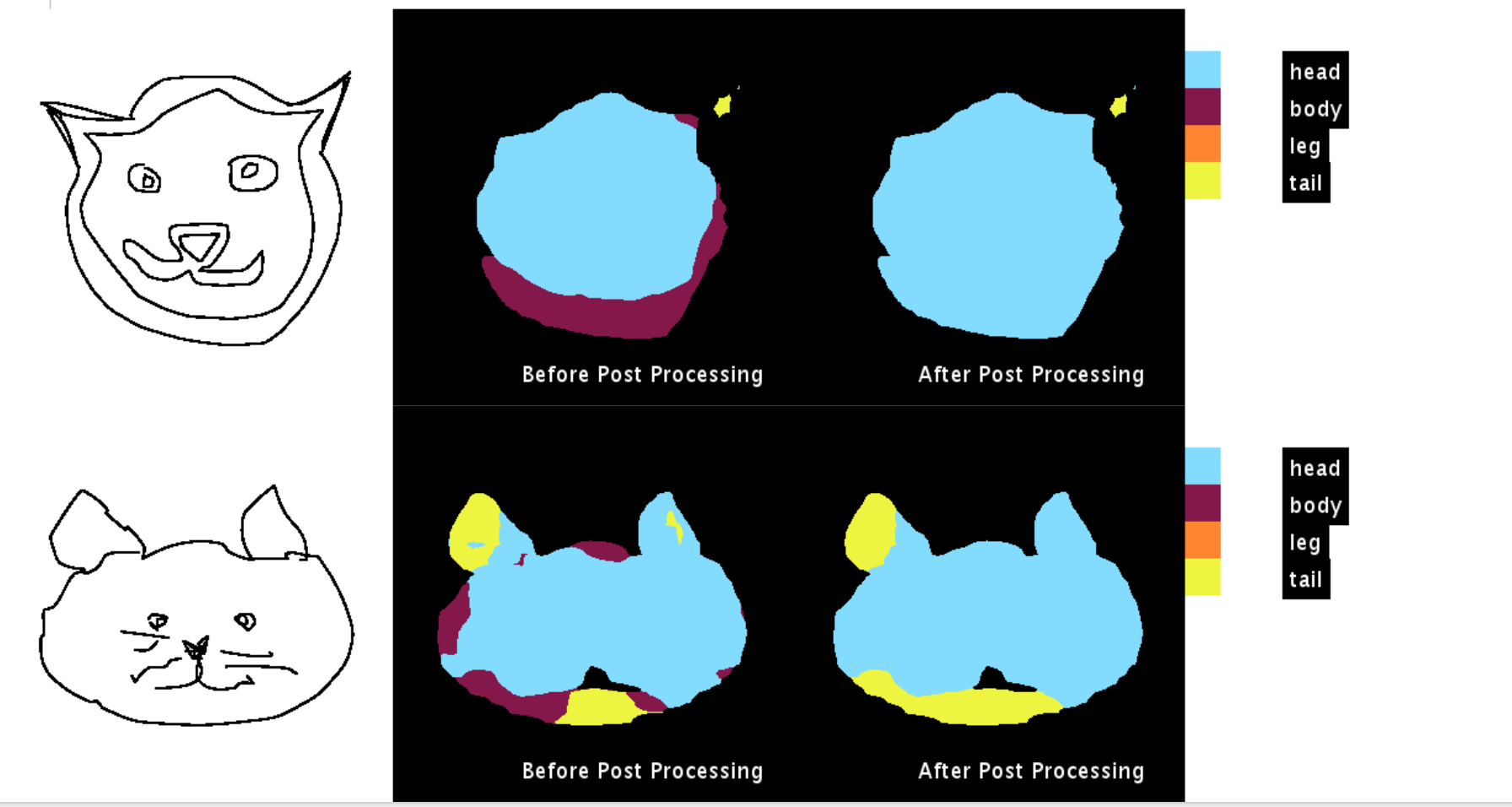
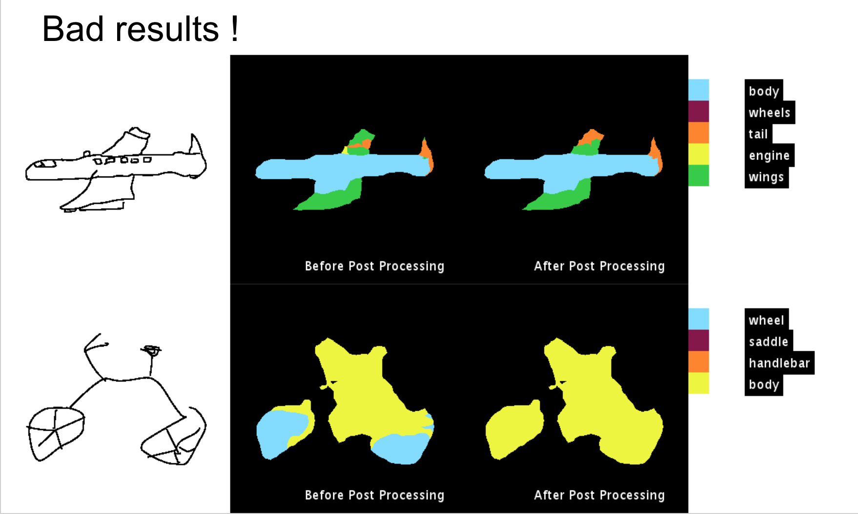
The code for the post processing method is available on github. The link to the repository is Understanding CRF’s using GMM

If any questions please feel free to contact me!

Cheers, Harsh Agarwal